Integration of two multi-omic datasets with (de)coupling
[1]:
import numpy as np
import scanpy as sc
import scvelo as scv
import torch
import matplotlib.pyplot as plt
import umap
import os
import multivelovae as vv
from datetime import datetime
[2]:
torch.cuda.is_available()
[2]:
True
[3]:
now = datetime.now()
date = now.strftime("%m_%d_%Y")
Read in processed data and define places to store output
[4]:
adata = sc.read_h5ad('3423-MV-2-8489-MV-1_adata_postpro_concat.h5ad')
adata_atac = sc.read_h5ad('3423-MV-2-8489-MV-1_adata_atac_postpro_concat.h5ad')
[5]:
gene_plot = ['AZU1', 'HBD', 'HDC', 'LYZ', 'PF4', 'SPINK2']
np.isin(gene_plot, adata.var_names)
[5]:
array([ True, True, True, True, True, True])
[6]:
'PROM1' in adata.var_names
[6]:
True
[7]:
dataset = "3423-MV-2-8489-MV-1"
model_path_base = f"checkpoints/{dataset}"
figure_path_base = f"figures/{dataset}"
data_path_base = f"data/{dataset}"
[8]:
adata, adata_atac
[8]:
(AnnData object with n_obs × n_vars = 17667 × 892
     obs: 'total_unspliced', 'total_spliced', 'log1p_total_unspliced', 'log1p_total_spliced', 'fraction_u', 'n_genes_by_counts', 'log1p_n_genes_by_counts', 'total_counts', 'log1p_total_counts', 'pct_counts_in_top_20_genes', 'total_counts_mt', 'log1p_total_counts_mt', 'pct_counts_mt', 'total_counts_rb', 'log1p_total_counts_rb', 'pct_counts_rb', 'total_counts_hla', 'log1p_total_counts_hla', 'pct_counts_hla', 'total_counts_hb', 'log1p_total_counts_hb', 'pct_counts_hb', 'outlier', 'initial_size_unspliced', 'initial_size_spliced', 'initial_size', 'n_counts', 'S_score', 'G2M_score', 'phase', 'CC_difference', 'total_unspliced2', 'total_spliced2', 'log1p_total_unspliced2', 'log1p_total_spliced2', 'fraction_u2', 'n_c', 'n_Mu', 'n_Ms', 'leiden', 'total_chromatin', 'total_unspliced3', 'total_spliced3', 'log1p_total_unspliced3', 'log1p_total_spliced3', 'fraction_u3', 'total_Mc', 'total_Mu', 'total_Ms', 'batch', 'n_Mc'
     var: 'gene_ids', 'feature_types', 'mt', 'rb', 'hla', 'hb', 'HVG-Sample 1', 'n_cells-Sample 1', 'n_cells_by_counts-Sample 1', 'mean_counts-Sample 1', 'log1p_mean_counts-Sample 1', 'pct_dropout_by_counts-Sample 1', 'total_counts-Sample 1', 'log1p_total_counts-Sample 1', 'gene_count_corr-Sample 1', 'highly_variable-Sample 1', 'mean-Sample 1', 'std-Sample 1', 'HVG-Sample 2', 'n_cells-Sample 2', 'n_cells_by_counts-Sample 2', 'mean_counts-Sample 2', 'log1p_mean_counts-Sample 2', 'pct_dropout_by_counts-Sample 2', 'total_counts-Sample 2', 'log1p_total_counts-Sample 2', 'gene_count_corr-Sample 2', 'highly_variable-Sample 2', 'mean-Sample 2', 'std-Sample 2'
     uns: 'batch_colors', 'leiden_colors', 'neighbors', 'umap'
     obsm: 'X_pca', 'X_umap'
     layers: 'Ms', 'Mu', 'spliced', 'spliced_raw', 'unspliced', 'unspliced_raw'
     obsp: 'connectivities', 'distances',
 AnnData object with n_obs × n_vars = 17667 × 892
     obs: 'n_counts', 'batch'
     layers: 'Mc', 'chromatin_raw')
[9]:
adata.obs['leiden'].cat.categories
[9]:
Index(['CMP', 'DC', 'Erythrocyte', 'GMP', 'Granulocyte', 'HSC', 'LMPP', 'MEP',
       'Mast Cells', 'Megakaryocyte', 'Platelet', 'Prog DC', 'Prog MK'],
      dtype='object')
[10]:
adata.obs['batch'].cat.categories
[10]:
Index(['Sample 1', 'Sample 2'], dtype='object')
[11]:
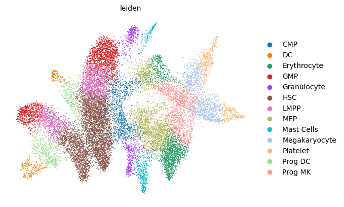
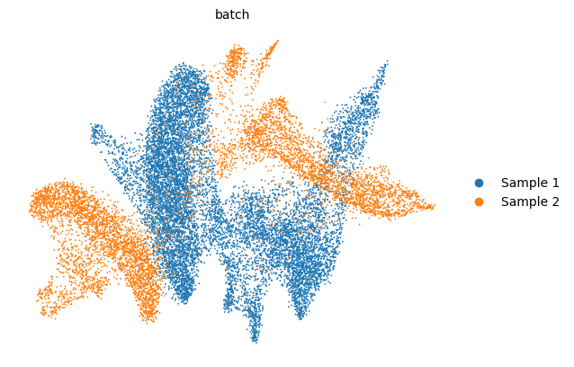
os.makedirs(figure_path_base, exist_ok=True)
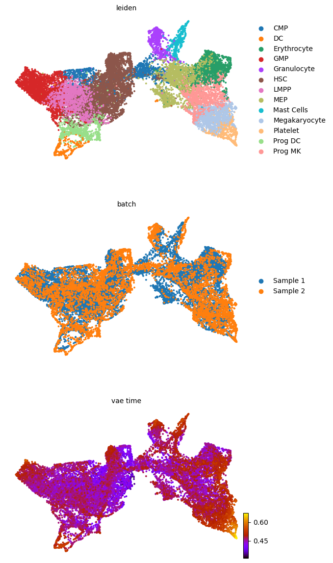
scv.pl.scatter(adata, basis='umap', color='leiden', legend_loc='right margin')
scv.pl.scatter(adata, basis='umap', color='batch', legend_loc='right margin')
[12]:
figure_path = figure_path_base+'/'+date
model_path = model_path_base+'/'+date
data_path = data_path_base
Initialize and train a MultiVeloVAE
[13]:
key = "vae"
[14]:
torch.manual_seed(2022)
np.random.seed(2022)
model = vv.VAEChrom(adata,
                    adata_atac,
                    batch_key='batch',
                    ref_batch=1,
                    batch_hvg_key='highly_variable',
                    var_to_regress=['total_unspliced3'],
                    device='cuda:0',
                    plot_init=False,
                    gene_plot=gene_plot,
                    cluster_key="leiden",
                    figure_path=figure_path,
                    embed="umap")

model.train(plot=False,
            gene_plot=gene_plot,
            figure_path=figure_path,
            embed="umap")

model.save_model(model_path)
model.save_anndata(data_path, file_name="out.h5ad")
CVAE enabled. Performing batch effect correction.
Reference batch set to 1 (Sample 2).
Latent dimension set to 8.
KL weights set to 2.00 2.00.
Found ['total_unspliced3'] in obs. Regressing them out.
Batch 0 sparsity: 0.118
Batch 1 sparsity: 0.139
Learning rate set to 7.4e-4 based on data sparsity.
Early stop threshold set to 1.5.
Using Gaussian Prior.
Initializing using the steady-state and dynamical models.
859 out of 892 = 96.3% genes have good ellipse fits.
KS-test result: [1. 1. 1. 1. 1. 1. 1.]
Assigning cluster 6 to repressive.
Initial induction: 690, repression: 202 out of 892.
Computing scaling factors for each batch class.
-------------------------- Train a MultiVeloVAE -------------------------
*********      Creating Training and Validation Datasets      *********
Total Number of Iterations Per Epoch: 49, test iteration: 96
*********                      Finished.                      *********
*********                      Stage  1                       *********
Epoch 1: Train ELBO = 122.456, Test ELBO = -58430.989           Total Time =   0 h :  0 m :  0 s
Epoch 50: Train ELBO = 1501.256, Test ELBO = 1497.321           Total Time =   0 h :  0 m : 16 s
*********     Stage 1: Early Stop Triggered at epoch 83.     *********
*********     Retrieving best model from iteration 3745.      *********
*********                      Stage  2                       *********
Cell-wise KNN estimation.
Using 618 latent neighbors to select ancestors.
Percentage of Invalid Sets: 0.000
Average Set Size: 80
Finished. Actual Time:   0 h :  0 m : 15 s
*********             Velocity Refinement Round 1             *********
Epoch 92: Train ELBO = 1502.394, Test ELBO = 1498.219           Total Time =   0 h :  0 m : 44 s
*********     Round 1: Early Stop Triggered at epoch 92.     *********
*********     Retrieving best model from iteration 4450.      *********
Cell-wise KNN estimation.
Finished. Actual Time:   0 h :  0 m :  2 s
*********             Velocity Refinement Round 2             *********
Epoch 96: Train ELBO = 1479.619, Test ELBO = 1475.280           Total Time =   0 h :  0 m : 48 s
*********     Round 2: Early Stop Triggered at epoch 96.     *********
*********     Retrieving best model from iteration 4642.      *********
Change in x0: 0.181
Cell-wise KNN estimation.
Finished. Actual Time:   0 h :  0 m :  2 s
*********             Velocity Refinement Round 3             *********
Epoch 100: Train ELBO = 1454.875, Test ELBO = 1451.734          Total Time =   0 h :  0 m : 52 s
*********     Round 3: Early Stop Triggered at epoch 100.     *********
*********     Retrieving best model from iteration 4834.      *********
Change in x0: 0.140
Cell-wise KNN estimation.
Finished. Actual Time:   0 h :  0 m :  2 s
*********             Velocity Refinement Round 4             *********
Epoch 104: Train ELBO = 1436.807, Test ELBO = 1434.346          Total Time =   0 h :  0 m : 55 s
*********     Round 4: Early Stop Triggered at epoch 104.     *********
*********     Retrieving best model from iteration 5026.      *********
Change in x0: 0.116
Cell-wise KNN estimation.
Finished. Actual Time:   0 h :  0 m :  2 s
*********             Velocity Refinement Round 5             *********
Epoch 108: Train ELBO = 1425.287, Test ELBO = 1423.135          Total Time =   0 h :  0 m : 59 s
*********     Round 5: Early Stop Triggered at epoch 108.     *********
*********     Retrieving best model from iteration 5218.      *********
Change in x0: 0.097
*********      Stage 2: Early Stop Triggered at round 5.      *********
Final: Train ELBO = 1425.287,   Test ELBO = 1423.135
*********      Finished. Total Time =   0 h :  1 m :  0 s     *********
Using reference batch for latent variable computation.
Computing velocity.
Selected 726 velocity genes.
Writing anndata output to file.
Downstream analyses
[15]:
z = adata.obsm[f'{key}_z']
t = adata.obs[f'{key}_time'].to_numpy()
rho = adata.layers[f'{key}_rho']
kc = adata.layers[f'{key}_kc']
[16]:
# UMAP embedding from latent cell space using reference label
umap_obj = umap.UMAP(n_neighbors=30, n_components=2, min_dist=0.25, random_state=2022)
z_umap = umap_obj.fit_transform(z)

# UMAP embedding from latent cell space using original batch labels
z_batch = adata.obsm[f'{key}_z_batch']
umap_obj = umap.UMAP(n_neighbors=30, n_components=2, min_dist=0.25, random_state=2022)
z_umap2 = umap_obj.fit_transform(z_batch)
[17]:
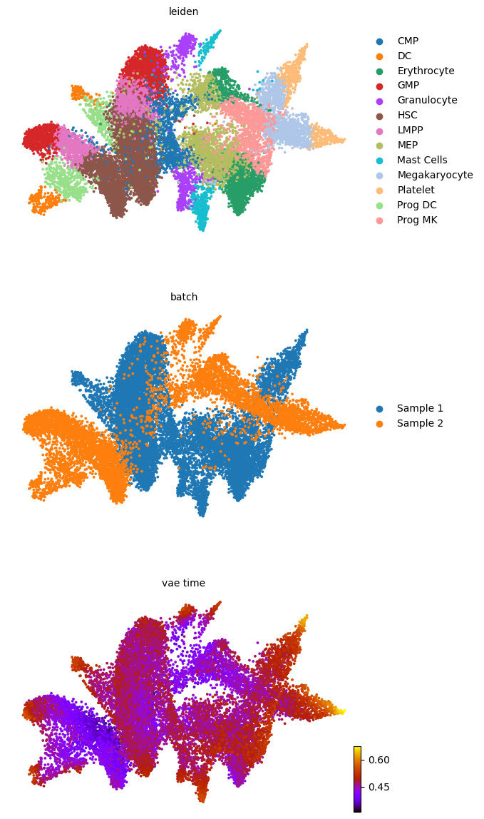
scv.pl.scatter(adata, basis='umap', color=['leiden', 'batch', f'{key}_time'], legend_loc='right', color_map='gnuplot', ncols=1, size=30)
adata.obsm['X_z_umap'] = z_umap
scv.pl.scatter(adata, basis='z_umap', color=['leiden', 'batch', f'{key}_time'], legend_loc='right', color_map='gnuplot', ncols=1, size=30, save=f'{figure_path}/{dataset}_z_batch_time_{key}.png')
adata.obsm['X_z_umap2'] = z_umap2
scv.pl.scatter(adata, basis='z_umap2', color=['leiden', 'batch', f'{key}_time'], legend_loc='right', color_map='gnuplot', ncols=1, size=30, save=f'{figure_path}/{dataset}_z_batch_time2_{key}.png')
saving figure to file figures/3423-MV-2-8489-MV-1/06_04_2025/3423-MV-2-8489-MV-1_z_batch_time_vae.png
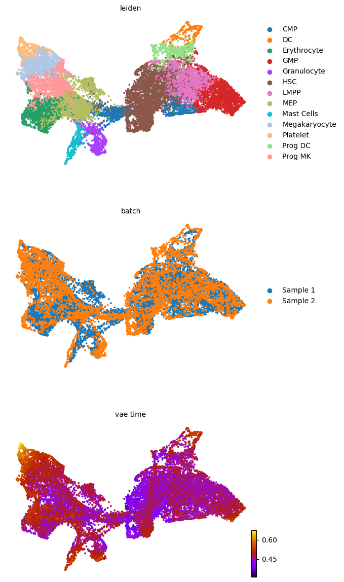
saving figure to file figures/3423-MV-2-8489-MV-1/06_04_2025/3423-MV-2-8489-MV-1_z_batch_time2_vae.png
[18]:
adata.obsm[f'{key}_latent'] = np.concatenate((adata.obsm[f'{key}_z'], adata.obsm[f'{key}_t']), axis=1)
sc.pp.neighbors(adata, use_rep=f'{key}_latent', n_neighbors=50)
[19]:
# Compute velocity graph on Z UMAP and visualize it, together with batch labels and inferred latent time
adata.obsm['X_z_umap'] = z_umap
vv.model.velocity_graph(adata, key=key, batch_corrected=True)
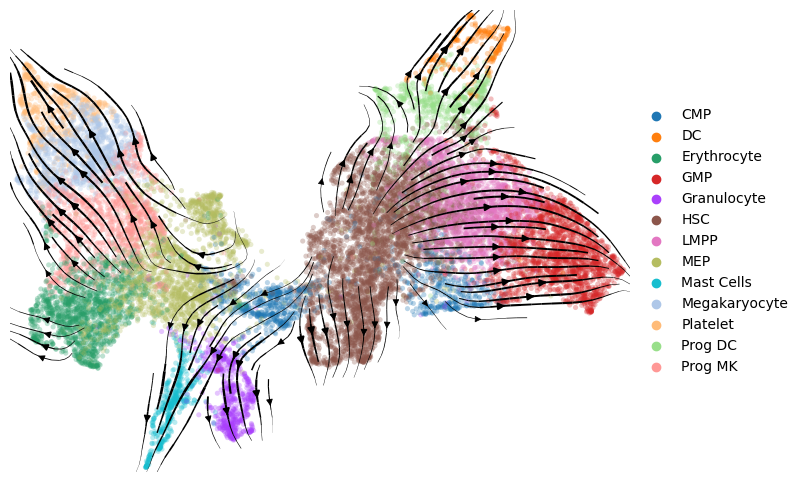
vv.velocity_embedding_stream(adata, key=key, basis='z_umap', color='leiden', title="", figsize=(8,6), legend_loc='right margin')
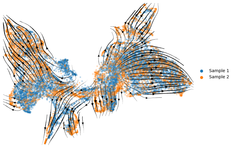
vv.velocity_embedding_stream(adata, key=key, basis='z_umap', color='batch', title="", figsize=(8,6), legend_loc='right margin')
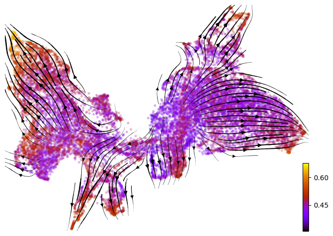
vv.velocity_embedding_stream(adata, key=key, basis='z_umap', color=f'{key}_time', color_map='gnuplot', title="", figsize=(8,6), legend_loc='right margin')
computing velocity graph (using 1/8 cores)
    finished (0:00:49) --> added
    'vae_velocity_norm_graph', sparse matrix with cosine correlations (adata.uns)
computing velocity embedding
    finished (0:00:02) --> added
    'vae_velocity_norm_z_umap', embedded velocity vectors (adata.obsm)
[20]:
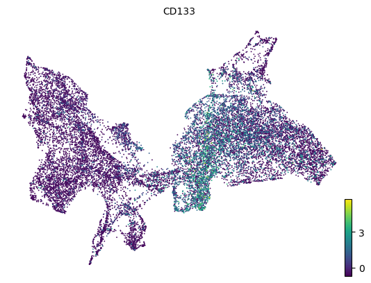
# HSC marker gene CD133 (PROM1)
scv.pl.scatter(adata, color='PROM1', basis='z_umap', title='CD133')
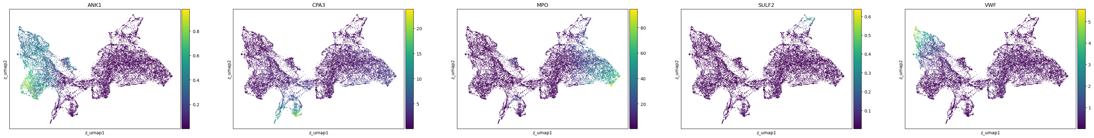
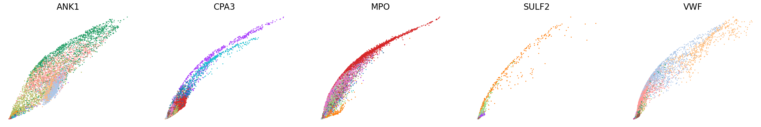
[21]:
sc.pl.scatter(adata, basis='z_umap', layers=f'{key}_shat', color=['ANK1', 'CPA3', 'MPO', 'SULF2', 'VWF'])
[22]:
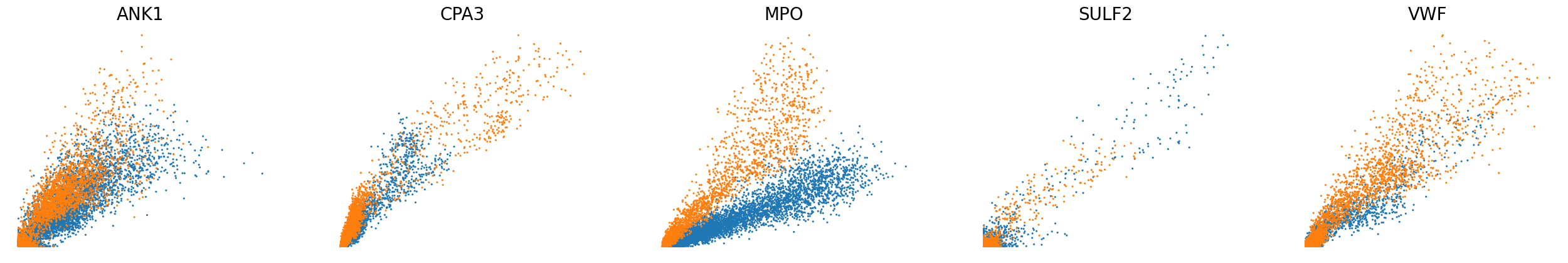
# Phase portraits of reconstructed unspliced and spliced levels
scv.pl.scatter(adata, basis=['ANK1', 'CPA3', 'MPO', 'SULF2', 'VWF'], color='batch', ncols=5, frameon=False, size=20, fontsize=20)
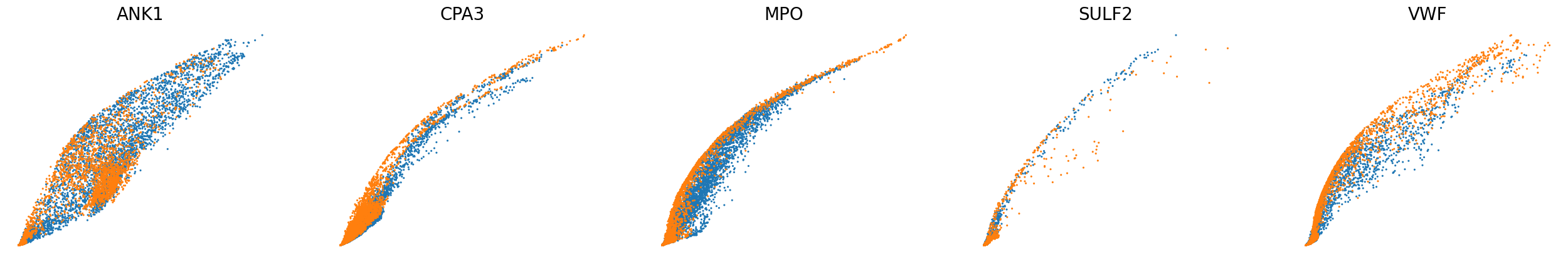
scv.pl.scatter(adata, basis=['ANK1', 'CPA3', 'MPO', 'SULF2', 'VWF'], x=f'{key}_shat', y=f'{key}_uhat', color='batch', ncols=5, frameon=False, size=20, fontsize=20)
scv.pl.scatter(adata, basis=['ANK1', 'CPA3', 'MPO', 'SULF2', 'VWF'], x=f'{key}_shat', y=f'{key}_uhat', color='leiden', ncols=5, frameon=False, size=20, fontsize=20)
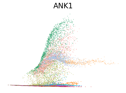
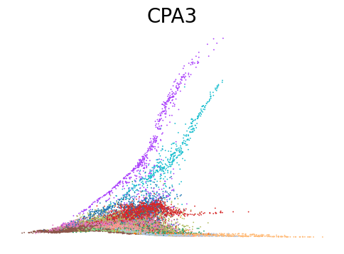
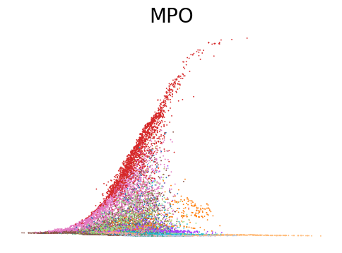
[23]:
# Dynamic plots of modality level by latent time for genes of interest
for gene in ['ANK1', 'CPA3', 'MPO', 'SULF2', 'VWF']:
    scv.pl.scatter(adata, x=adata.obs[f'{key}_time'], y=adata[:, gene].layers[f'{key}_shat'], color='leiden', figsize=(6,4), title=f'{gene}', legend_loc='none', frameon=False, fontsize=20)
Decoupling and coupling factors of cells
[24]:
import matplotlib.colors as mcolors
[25]:
adata.layers[f'{key}_decoupling'] = adata.layers[f'{key}_kc'] - adata.layers[f'{key}_rho']
adata.layers[f'{key}_coupling'] = adata.layers[f'{key}_kc'] + adata.layers[f'{key}_rho'] - 1
[26]:
# Decouping factors of each modality on dynamic plots
scv.pl.scatter(adata, basis=['AZU1', 'HBD', 'HDC', 'LYZ', 'PF4', 'SPINK2'], x=f'{key}_time', y=f'{key}_chat', color=f'{key}_decoupling', dpi=300, legend_loc='none', frameon=False, fontsize=30, color_map='coolwarm', size=40,
               norm=mcolors.CenteredNorm(halfrange=1), colorbar=False, wspace=0.1)
scv.pl.scatter(adata, basis=['AZU1', 'HBD', 'HDC', 'LYZ', 'PF4', 'SPINK2'], x=f'{key}_time', y=f'{key}_uhat', color=f'{key}_decoupling', dpi=300, legend_loc='none', frameon=False, fontsize=30, color_map='coolwarm', size=40,
               norm=mcolors.CenteredNorm(halfrange=1), colorbar=False, wspace=0.1)
scv.pl.scatter(adata, basis=['AZU1', 'HBD', 'HDC', 'LYZ', 'PF4', 'SPINK2'], x=f'{key}_time', y=f'{key}_shat', color=f'{key}_decoupling', dpi=300, legend_loc='none', frameon=False, fontsize=30, color_map='coolwarm', size=40,
               norm=mcolors.CenteredNorm(halfrange=1), colorbar=False, wspace=0.1)
[27]:
# Couping factors of each modality on dynamic plots
scv.pl.scatter(adata, basis=['AZU1', 'HBD', 'HDC', 'LYZ', 'PF4', 'SPINK2'], x=f'{key}_time', y=f'{key}_chat', color=f'{key}_coupling', dpi=300, legend_loc='none', frameon=False, fontsize=30, color_map='coolwarm', size=40,
               norm=mcolors.CenteredNorm(halfrange=1), colorbar=False, wspace=0.1)
scv.pl.scatter(adata, basis=['AZU1', 'HBD', 'HDC', 'LYZ', 'PF4', 'SPINK2'], x=f'{key}_time', y=f'{key}_uhat', color=f'{key}_coupling', dpi=300, legend_loc='none', frameon=False, fontsize=30, color_map='coolwarm', size=40,
               norm=mcolors.CenteredNorm(halfrange=1), colorbar=False, wspace=0.1)
scv.pl.scatter(adata, basis=['AZU1', 'HBD', 'HDC', 'LYZ', 'PF4', 'SPINK2'], x=f'{key}_time', y=f'{key}_shat', color=f'{key}_coupling', dpi=300, legend_loc='none', frameon=False, fontsize=30, color_map='coolwarm', size=40,
               norm=mcolors.CenteredNorm(halfrange=1), colorbar=False, wspace=0.1)
Plot phase portraits of genes with the highest likelihoods
[28]:
top_genes = adata[:, adata.var[f'{key}_velocity_genes']].var[f'{key}_likelihood'].sort_values(ascending=False).index
top_genes = top_genes[~np.isin(top_genes, ['ANK1', 'CPA3', 'MPO', 'SULF2', 'VWF'])]
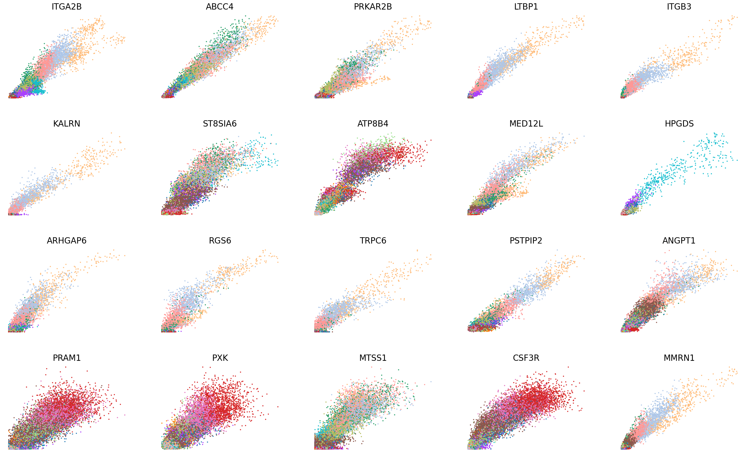
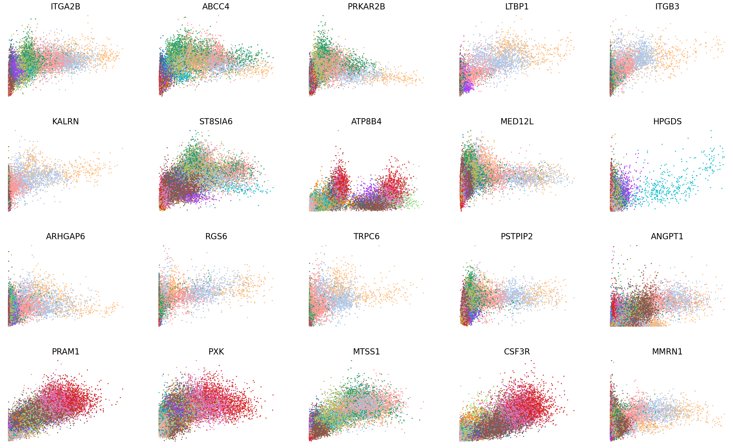
[29]:
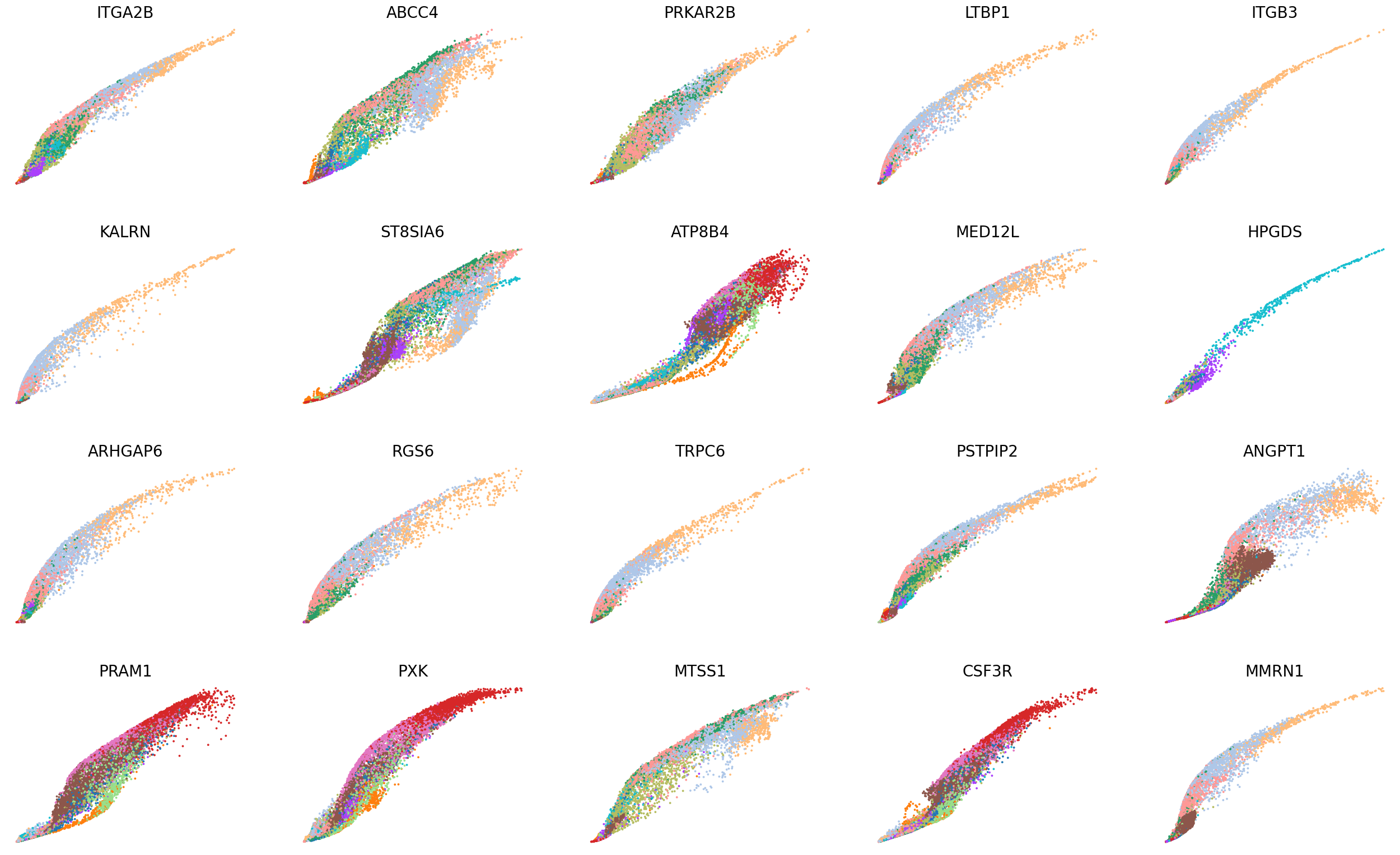
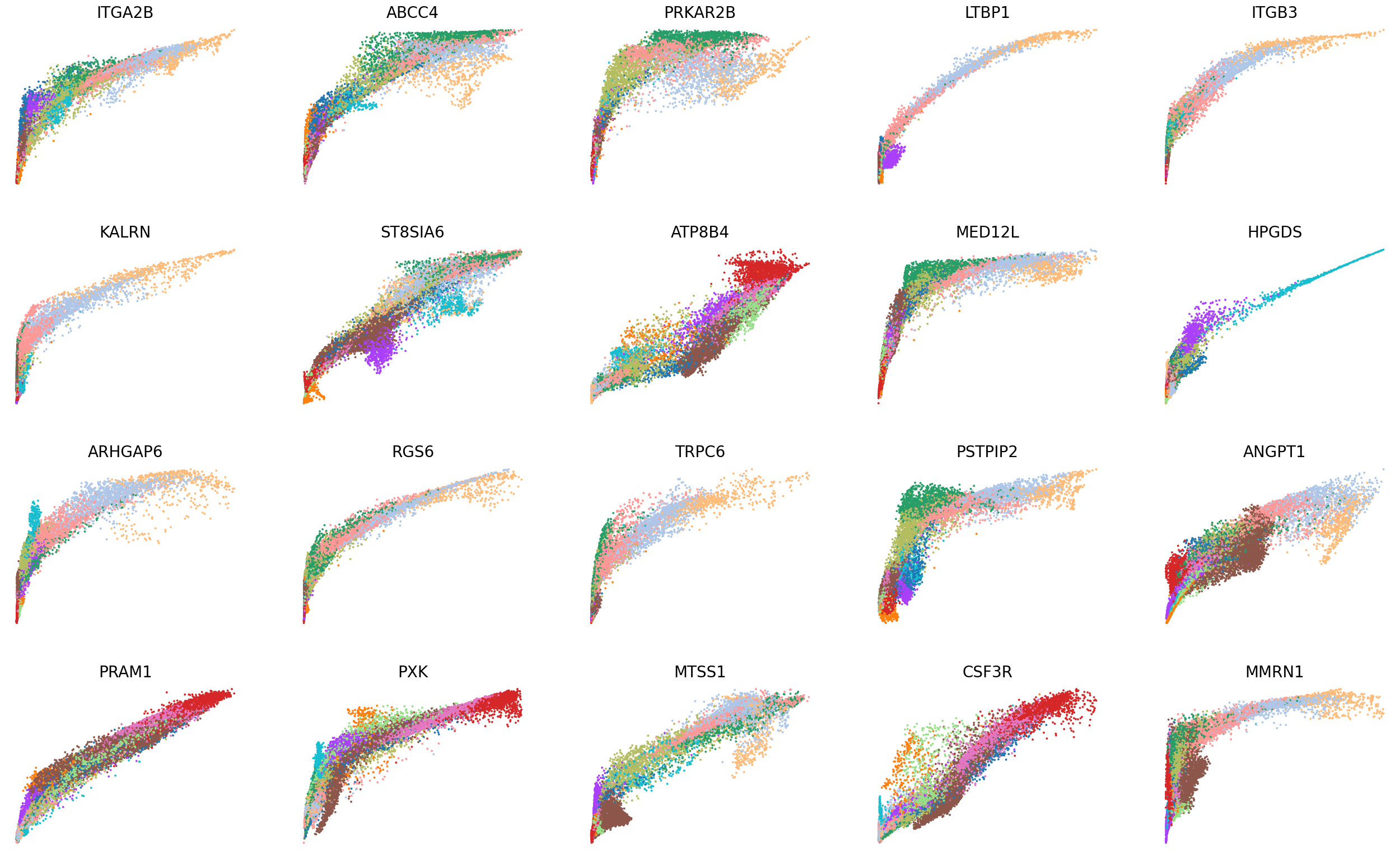
scv.pl.scatter(adata, basis=top_genes[:20], color='leiden', ncols=5, frameon=False, fontsize=20, size=30)
scv.pl.scatter(adata, basis=top_genes[:20], x=f'{key}_shat', y=f'{key}_uhat', color='leiden', ncols=5, frameon=False, fontsize=20, size=30)
[30]:
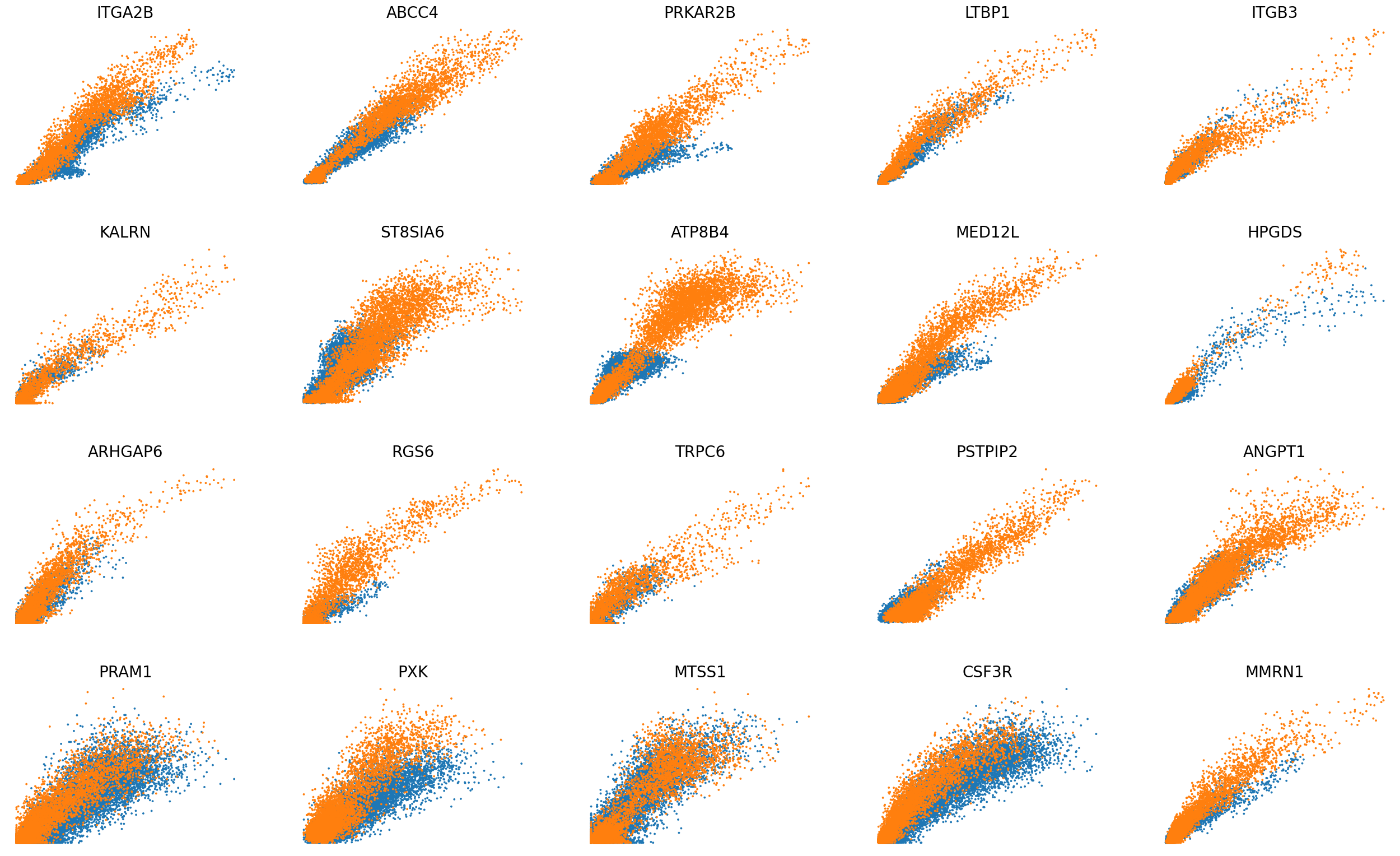
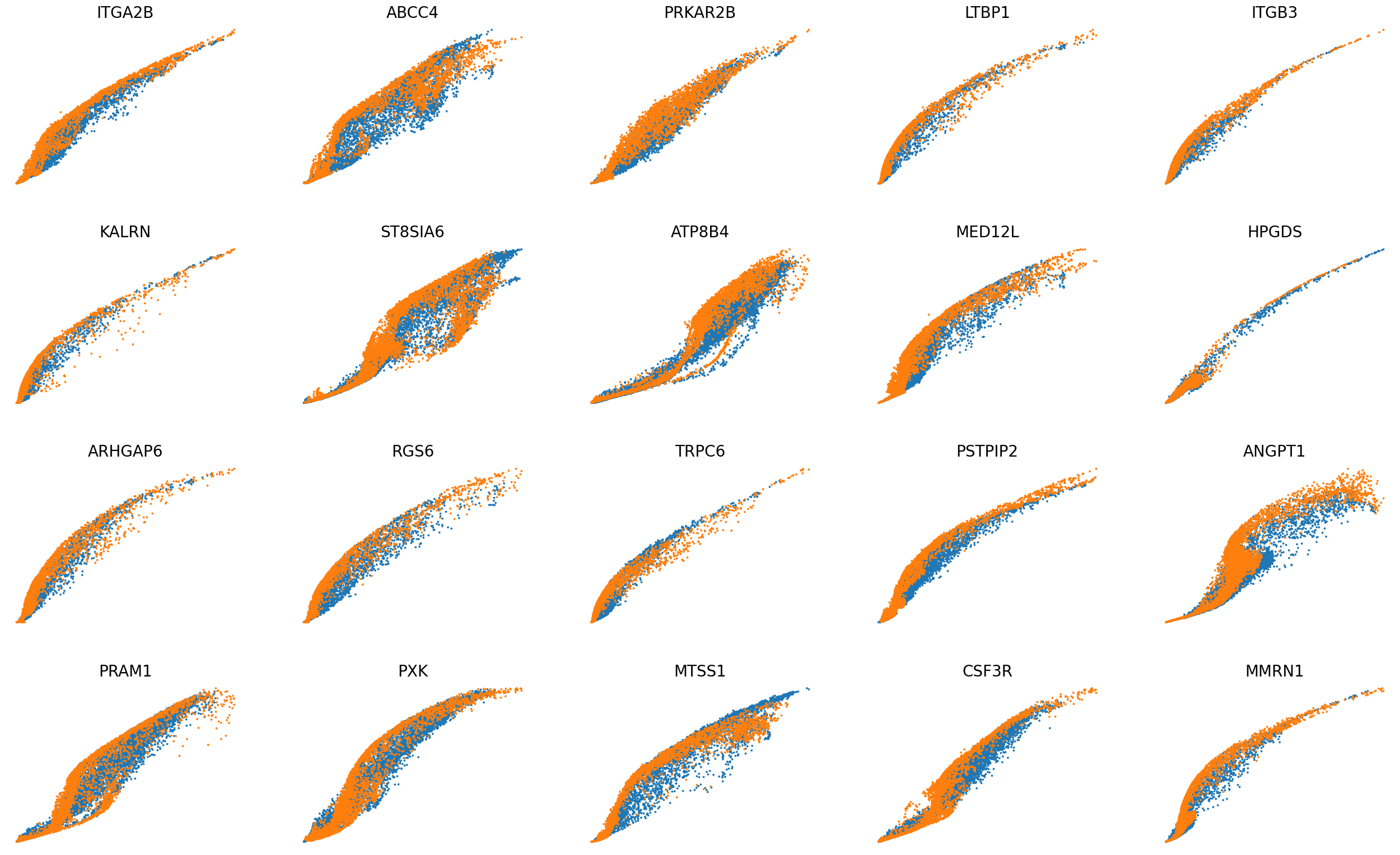
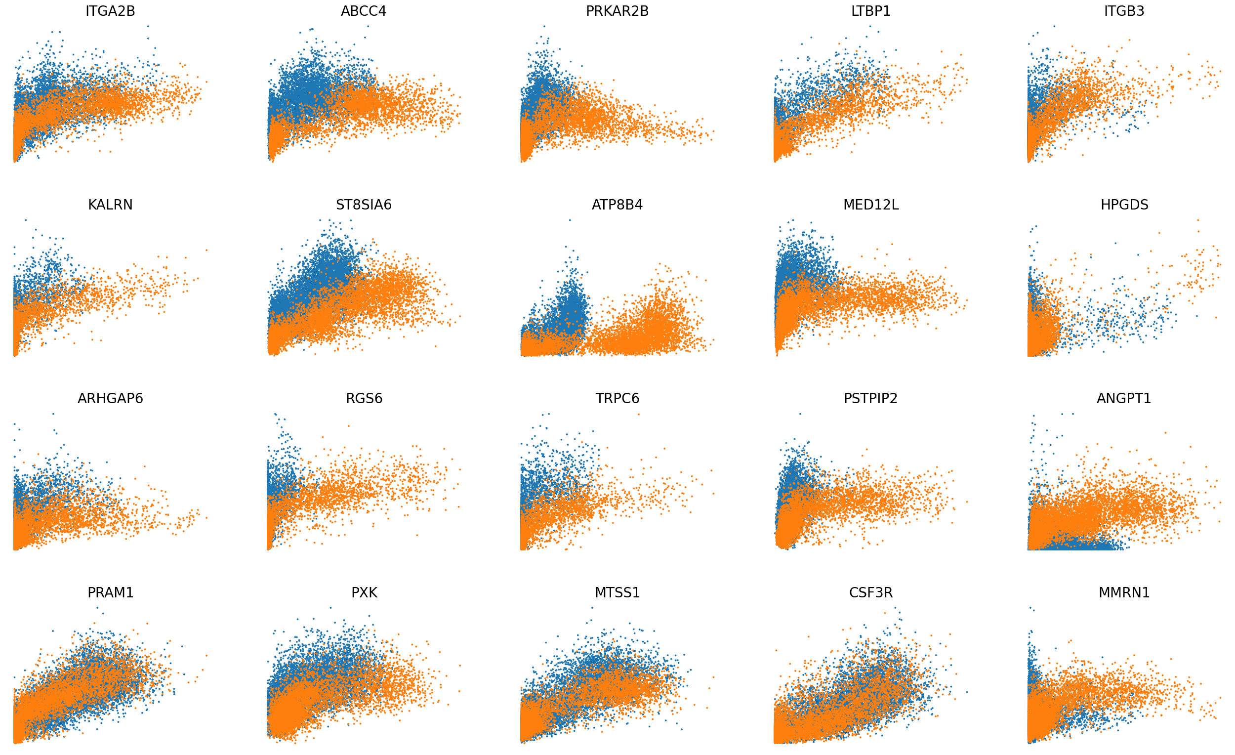
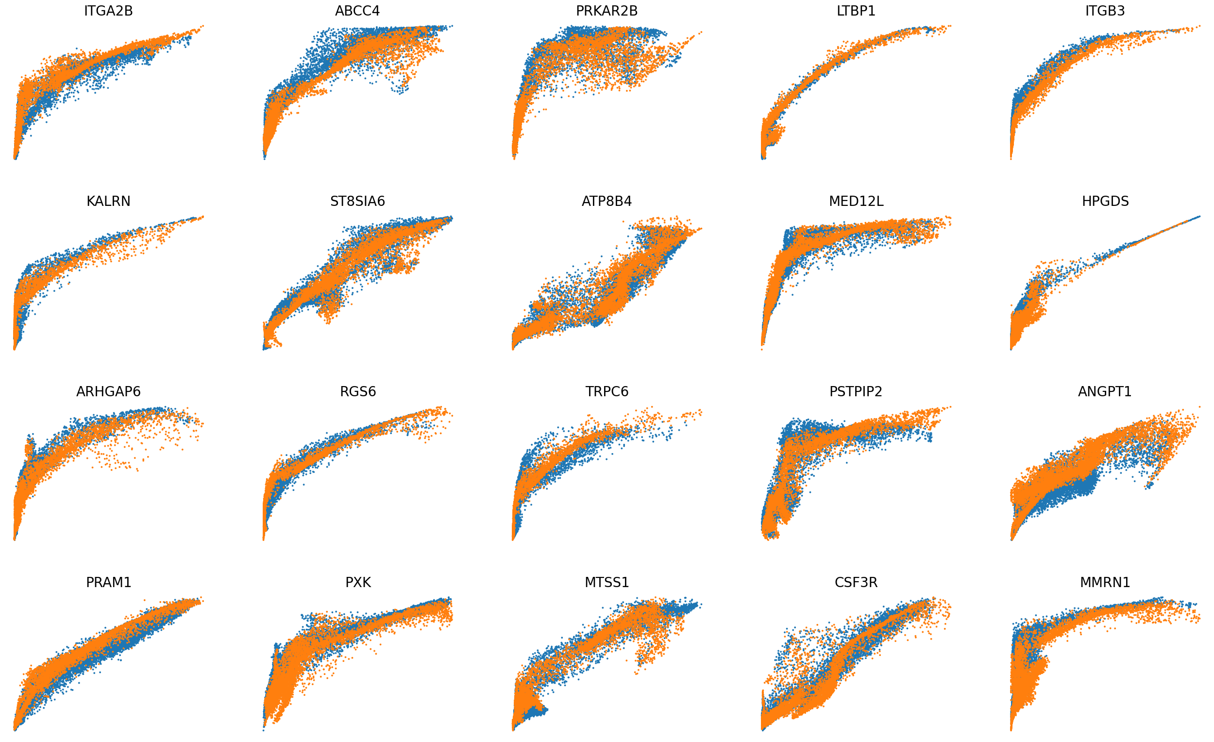
## Phase portraits compare before and after integration
scv.pl.scatter(adata, basis=top_genes[:20], color='batch', ncols=5, frameon=False, fontsize=20, size=30)
scv.pl.scatter(adata, basis=top_genes[:20], x=f'{key}_shat', y=f'{key}_uhat', color='batch', ncols=5, frameon=False, fontsize=20, size=30)
[31]:
adata.layers['Mc'] = adata_atac.layers['Mc'].copy()
[32]:
scv.pl.scatter(adata, basis=top_genes[:20], x='Mu', y='Mc', color='leiden', ncols=5, frameon=False, fontsize=20, size=30)
scv.pl.scatter(adata, basis=top_genes[:20], x=f'{key}_uhat', y=f'{key}_chat', color='leiden', ncols=5, frameon=False, fontsize=20, size=30)
[33]:
scv.pl.scatter(adata, basis=top_genes[:20], x='Mu', y='Mc', color='batch', ncols=5, frameon=False, fontsize=20, size=30)
scv.pl.scatter(adata, basis=top_genes[:20], x=f'{key}_uhat', y=f'{key}_chat', color='batch', ncols=5, frameon=False, fontsize=20, size=30)
[34]:
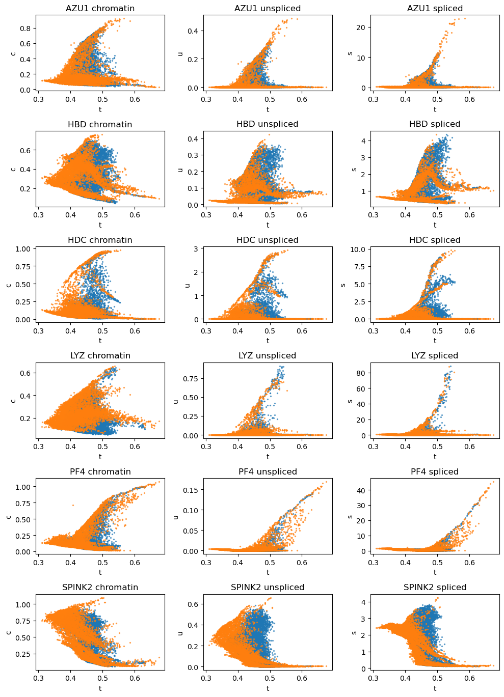
# Dynamic plots of several marker genes colored by batch labels
vv.dynamic_plot(adata, adata_atac, gene_plot, color_by='batch', batch_correction=True)
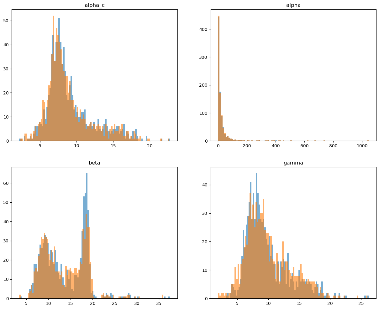
Distributions of inferred rate parameters
[35]:
fig, axs = plt.subplots(2, 2, figsize=(15, 12))
axs[0, 0].hist(adata.var[f'{key}_alpha_c_0'], bins=100, alpha=0.6);
axs[0, 0].hist(adata.var[f'{key}_alpha_c_1'], bins=100, alpha=0.6);
axs[0, 0].set_title('alpha_c');
a1 = adata.var[f'{key}_alpha_0'].values
a1 = a1[a1 < np.percentile(a1, 99.5)]
a2 = adata.var[f'{key}_alpha_1'].values
a2 = a2[a2 < np.percentile(a2, 99.5)]
axs[0, 1].hist(a1, bins=100, alpha=0.6);
axs[0, 1].hist(a2, bins=100, alpha=0.6);
axs[0, 1].set_title('alpha');
axs[1, 0].hist(adata.var[f'{key}_beta_0'], bins=100, alpha=0.6);
axs[1, 0].hist(adata.var[f'{key}_beta_1'], bins=100, alpha=0.6);
axs[1, 0].set_title('beta');
axs[1, 1].hist(adata.var[f'{key}_gamma_0'], bins=100, alpha=0.6);
axs[1, 1].hist(adata.var[f'{key}_gamma_1'], bins=100, alpha=0.6);
axs[1, 1].set_title('gamma');
Save the final result
[36]:
adata.write_h5ad(data_path_base+"/final.h5ad")
[ ]: