Single scRNA-seq dataset
[1]:
import numpy as np
import scanpy as sc
import scvelo as scv
import torch
import matplotlib.pyplot as plt
import umap
import os
import multivelovae as vv
from datetime import datetime
import seaborn as sns
import pandas as pd
[2]:
torch.cuda.is_available()
[2]:
True
[3]:
now = datetime.now()
date = now.strftime("%m_%d_%Y")
Read in processed data and define places to store output
[4]:
dataset = "VV_braindev"
adata = sc.read_h5ad('Braindev_post.h5ad')
[5]:
model_path_base = f"checkpoints/{dataset}"
figure_path_base = f"figures/{dataset}"
data_path_base = f"data/{dataset}"
[6]:
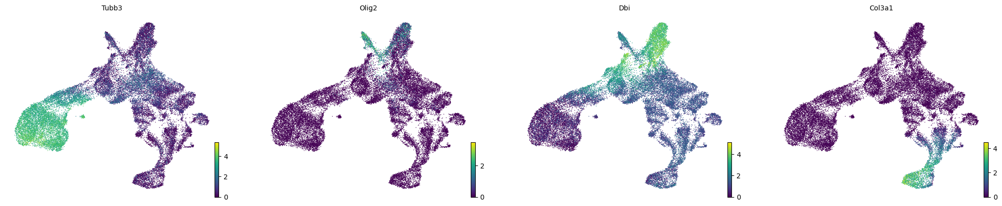
gene_plot = ['Tubb3', 'Olig2', 'Dbi', 'Col3a1']
np.all(np.isin(gene_plot, adata.var_names))
[6]:
True
[7]:
adata
[7]:
AnnData object with n_obs × n_vars = 29948 × 2000
    obs: 'Age', 'CellCycle', 'Cell_Conc', 'Chemistry', 'ChipID', 'Class', 'ClusterName', 'Clusters', 'Date_Captured', 'DonorID', 'DoubletFinderPCA', 'HPF_LogPP', 'IsCycling', 'Label', 'Location_E9_E11', 'NCellsCluster', 'NGenes', 'Num_Pooled_Animals', 'PCR_Cycles', 'Plug_Date', 'Project', 'PseudoAge', 'PseudoTissue', 'Region', 'SampleID', 'SampleName', 'Sample_Index', 'Sex', 'Species', 'Split', 'Strain', 'Subclass', 'Target_Num_Cells', 'Tissue', 'TotalUMI', 'Transcriptome', 'cDNA_Lib_Ok', 'ngperul_cDNA', 'tprior', 'clusters', 'n_counts', 'n_genes', 'initial_size_spliced', 'initial_size_unspliced', 'initial_size', 'velovae_time', 'velovae_std_t', 'velovae_t0', 'fullvb_time', 'fullvb_std_t', 'fullvb_t0', 'velovae_velocity_consistency', 'velovae_velocity_self_transition', 'fullvb_velocity_consistency', 'fullvb_velocity_self_transition'
    var: 'Accession', 'Chromosome', 'End', 'Gamma', 'Selected', 'Start', 'Strand', 'Valid', 'gene_count_corr', 'means', 'dispersions', 'dispersions_norm', 'highly_variable', 'w_init', 'velovae_alpha', 'velovae_beta', 'velovae_gamma', 'velovae_ton', 'velovae_scaling', 'velovae_sigma_u', 'velovae_sigma_s', 'fullvb_logmu_alpha', 'fullvb_logmu_beta', 'fullvb_logmu_gamma', 'fullvb_logstd_alpha', 'fullvb_logstd_beta', 'fullvb_logstd_gamma', 'fullvb_ton', 'fullvb_scaling', 'fullvb_sigma_u', 'fullvb_sigma_s', 'velocity_genes', 'velovae_mse_train', 'velovae_mse_test', 'velovae_mae_train', 'velovae_mae_test', 'velovae_likelihood_train', 'velovae_likelihood_test', 'fullvb_mse_train', 'fullvb_mse_test', 'fullvb_mae_train', 'fullvb_mae_test', 'fullvb_likelihood_train', 'fullvb_likelihood_test'
    uns: 'clusters_colors', 'fullvb_run_time', 'fullvb_test_idx', 'fullvb_train_idx', 'fullvb_velocity_graph', 'fullvb_velocity_graph_neg', 'fullvb_velocity_params', 'neighbors', 'umap', 'velovae_run_time', 'velovae_test_idx', 'velovae_train_idx', 'velovae_velocity_graph', 'velovae_velocity_graph_neg', 'velovae_velocity_params'
    obsm: 'BTSNE', 'HPF', 'HPF_theta', 'PCA', 'TSNE', 'UMAP', 'UMAP3D', 'X_pca', 'X_tsne', 'X_umap', 'fullvb_std_z', 'fullvb_velocity_umap', 'fullvb_z', 'velovae_std_z', 'velovae_velocity_umap', 'velovae_z', 'z_umap'
    varm: 'HPF', 'HPF_beta', 'MultilevelMarkers', 'fullvb_mode', 'velovae_mode'
    layers: 'Ms', 'Mu', 'expected', 'fullvb_rho', 'fullvb_s0', 'fullvb_shat', 'fullvb_u0', 'fullvb_uhat', 'fullvb_velocity', 'fullvb_velocity_u', 'matrix', 'pooled', 'spliced', 'unspliced', 'velovae_rho', 'velovae_s0', 'velovae_shat', 'velovae_u0', 'velovae_uhat', 'velovae_velocity', 'velovae_velocity_u'
    obsp: 'connectivities', 'distances'
[8]:
os.makedirs(figure_path_base, exist_ok=True)
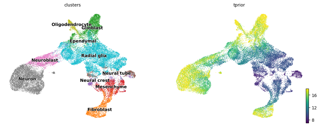
scv.pl.scatter(adata, basis='umap', color=['clusters', 'tprior'], legend_loc='on data')
[9]:
scv.pl.scatter(adata, basis='umap', color=gene_plot)
[10]:
figure_path = figure_path_base+'/'+date
model_path = model_path_base+'/'+date
data_path = data_path_base
Initialize and train a MultiVeloVAE
[11]:
key = 'vae'
[12]:
torch.manual_seed(2022)
np.random.seed(2022)
model = vv.VAEChrom(adata,
                    device='cuda:0',
                    plot_init=False,
                    gene_plot=gene_plot,
                    cluster_key="clusters",
                    figure_path=figure_path,
                    embed="umap")

model.train(plot=False,
            gene_plot=gene_plot,
            figure_path=figure_path,
            embed="umap")

model.save_model(model_path)
model.save_anndata(data_path, file_name="out.h5ad")
Running in RNA-only mode.
Latent dimension set to 6.
Learning rate set to 3.6e-4 based on data sparsity.
Early stop threshold set to 1.0.
Using Gaussian Prior.
Initializing using the steady-state and dynamical models.
1342 out of 2000 = 67.1% genes have good ellipse fits.
KS-test result: [0. 1. 1. 1. 1. 1. 1.]
Initial induction: 1567, repression: 433 out of 2000.
-------------------------- Train a MultiVeloVAE -------------------------
*********      Creating Training and Validation Datasets      *********
Total Number of Iterations Per Epoch: 82, test iteration: 162
*********                      Finished.                      *********
*********                      Stage  1                       *********
Epoch 1: Train ELBO = 1759.010, Test ELBO = -28886.076          Total Time =   0 h :  0 m :  1 s
Epoch 50: Train ELBO = 4616.443, Test ELBO = 4619.623           Total Time =   0 h :  0 m : 31 s
Epoch 100: Train ELBO = 4678.848, Test ELBO = 4680.425          Total Time =   0 h :  1 m :  2 s
Epoch 150: Train ELBO = 4701.216, Test ELBO = 4701.297          Total Time =   0 h :  1 m : 33 s
Epoch 200: Train ELBO = 4712.558, Test ELBO = 4714.119          Total Time =   0 h :  2 m :  4 s
Epoch 250: Train ELBO = 4722.968, Test ELBO = 4724.892          Total Time =   0 h :  2 m : 34 s
*********     Stage 1: Early Stop Triggered at epoch 295.     *********
*********     Retrieving best model from iteration 24139.      *********
*********                      Stage  2                       *********
Cell-wise KNN estimation.
Using 1000 latent neighbors to select ancestors.
Percentage of Invalid Sets: 0.002
Average Set Size: 102
Finished. Actual Time:   0 h :  0 m : 31 s
*********             Velocity Refinement Round 1             *********
Epoch 344: Train ELBO = 4676.564, Test ELBO = 4691.253          Total Time =   0 h :  4 m :  2 s
*********     Round 1: Early Stop Triggered at epoch 344.     *********
*********     Retrieving best model from iteration 28109.      *********
Cell-wise KNN estimation.
Finished. Actual Time:   0 h :  0 m :  4 s
*********             Velocity Refinement Round 2             *********
Epoch 492: Train ELBO = 4391.590, Test ELBO = 4381.878          Total Time =   0 h :  5 m : 33 s
*********     Round 2: Early Stop Triggered at epoch 492.     *********
*********     Retrieving best model from iteration 40178.      *********
Change in x0: 0.244
Cell-wise KNN estimation.
Finished. Actual Time:   0 h :  0 m :  4 s
*********             Velocity Refinement Round 3             *********
Epoch 637: Train ELBO = 4325.737, Test ELBO = 4311.295          Total Time =   0 h :  7 m :  3 s
*********     Round 3: Early Stop Triggered at epoch 637.     *********
*********     Retrieving best model from iteration 52004.      *********
Change in x0: 0.220
Cell-wise KNN estimation.
Finished. Actual Time:   0 h :  0 m :  4 s
*********             Velocity Refinement Round 4             *********
Epoch 644: Train ELBO = 4507.058, Test ELBO = 4502.342          Total Time =   0 h :  7 m : 13 s
*********     Round 4: Early Stop Triggered at epoch 644.     *********
*********     Retrieving best model from iteration 52490.      *********
Change in x0: 0.173
Cell-wise KNN estimation.
Finished. Actual Time:   0 h :  0 m :  4 s
*********             Velocity Refinement Round 5             *********
Epoch 651: Train ELBO = 4594.820, Test ELBO = 4593.610          Total Time =   0 h :  7 m : 22 s
*********     Round 5: Early Stop Triggered at epoch 651.     *********
*********     Retrieving best model from iteration 53138.      *********
Change in x0: 0.127
Cell-wise KNN estimation.
Finished. Actual Time:   0 h :  0 m :  4 s
*********             Velocity Refinement Round 6             *********
Epoch 658: Train ELBO = 4606.898, Test ELBO = 4605.955          Total Time =   0 h :  7 m : 32 s
*********     Round 6: Early Stop Triggered at epoch 658.     *********
*********     Retrieving best model from iteration 53705.      *********
Change in x0: 0.091
Final: Train ELBO = 4606.898,   Test ELBO = 4605.955
*********      Finished. Total Time =   0 h :  7 m : 32 s     *********
Computing velocity.
Selected 1337 velocity genes.
Writing anndata output to file.
Downstream analyses
[13]:
std_z = adata.obsm[f"{key}_std_z"]
z = adata.obsm[f"{key}_z"]
[14]:
# UMAP embedding from latent cell space
umap_obj = umap.UMAP(n_neighbors=30, n_components=2, min_dist=0.25, random_state=2022)
z_umap = umap_obj.fit_transform(z)
[15]:
# Compute velocity graph and visualize it, together with inferred latent time
vv.model.velocity_graph(adata, key=key)
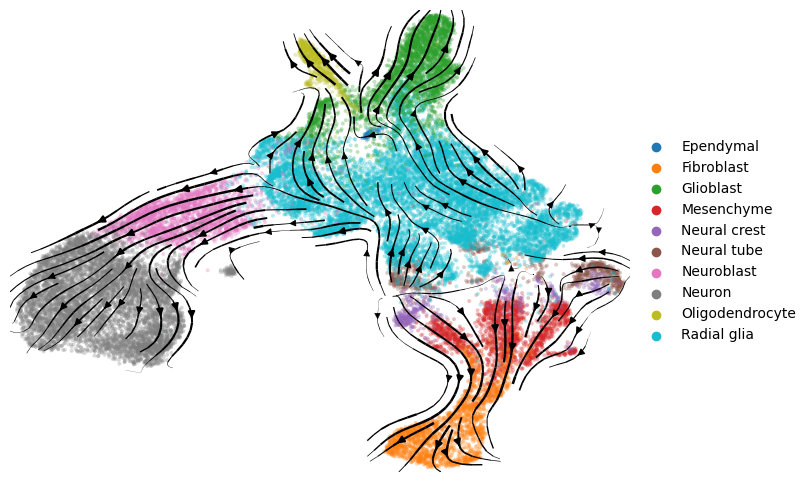
vv.velocity_embedding_stream(adata, key=key, basis='umap', color='clusters', title="", figsize=(8,6), legend_loc='right margin')
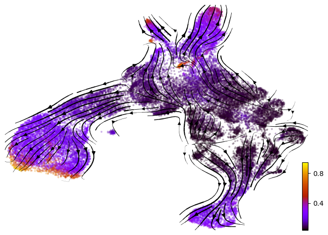
vv.velocity_embedding_stream(adata, key=key, basis='umap', color=f'{key}_time', color_map='gnuplot', title="", figsize=(8,6), legend_loc='right margin')
computing velocity graph (using 1/8 cores)
    finished (0:01:02) --> added
    'vae_velocity_norm_graph', sparse matrix with cosine correlations (adata.uns)
computing velocity embedding
    finished (0:00:03) --> added
    'vae_velocity_norm_umap', embedded velocity vectors (adata.obsm)
[16]:
# Compute cell state uncertainty
z_norm = np.linalg.norm(z, axis=1).reshape(-1, 1) + 1e-10
diff_entropy = np.sum(np.log(std_z/z_norm), 1) + 0.5*std_z.shape[1]*(1+np.log(2*np.pi))
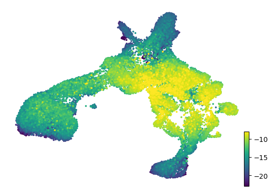
adata.obs['diff_entropy'] = diff_entropy
scv.pl.umap(adata, color='diff_entropy', size=30, title='', legend_loc='right margin', perc=[1, 99])
[17]:
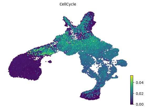
# Plot cell cycle
scv.pl.umap(adata, color='CellCycle', size=30)
[18]:
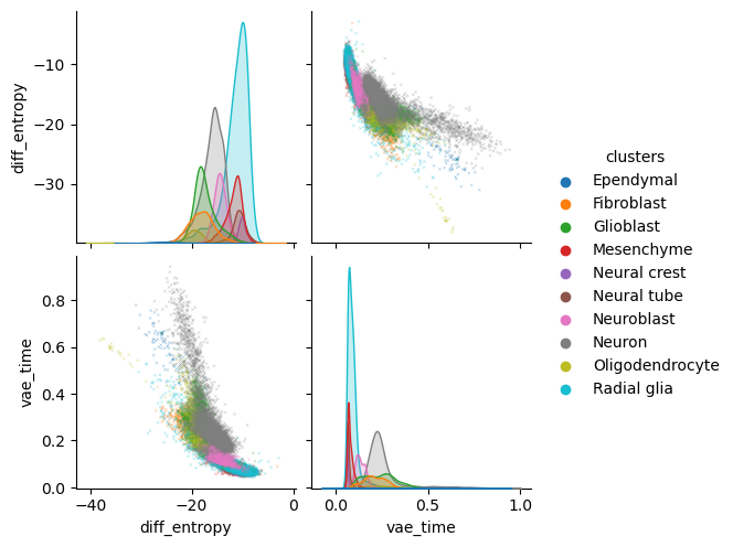
# Pairplot of uncertainty, latent time, and cell types
sns.pairplot(adata.obs[['diff_entropy', 'vae_time', 'clusters']], hue='clusters', palette='tab10', plot_kws={"s": 3, "alpha": 0.9}, markers='x');
[19]:
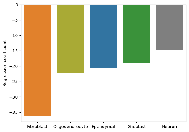
# Get the regression coefficients of uncertainty vs. latent time
slopes, intercepts = [], []
for cluster in adata.obs['clusters'].cat.categories:
    cluster_diff_entropy = adata.obs['diff_entropy'][adata.obs['clusters'] == cluster]
    cluster_time = adata.obs['vae_time'][adata.obs['clusters'] == cluster]
    slope, intercept = np.polyfit(cluster_time, cluster_diff_entropy, 1)
    slopes.append(slope)
    intercepts.append(intercept)

slope_df = pd.DataFrame({'clusters': adata.obs['clusters'].cat.categories, 'regression coefficient': slopes})
slope_df = slope_df.sort_values('regression coefficient')
slope_df = slope_df.loc[np.isin(slope_df['clusters'], ['Ependymal', 'Fibroblast', 'Glioblast', 'Neuron', 'Oligodendrocyte']),:]
fig, ax = plt.subplots(figsize=(7, 5))
color_map = {x:y for x,y in zip(adata.obs['clusters'].cat.categories, adata.uns['clusters_colors'])}
colors = [color_map[x] for x in slope_df['clusters']]
sns.barplot(data=slope_df, x='clusters', y='regression coefficient', palette=colors, ax=ax);
ax.set_xlabel('');
ax.set_ylabel('Regression coefficient');
[20]:
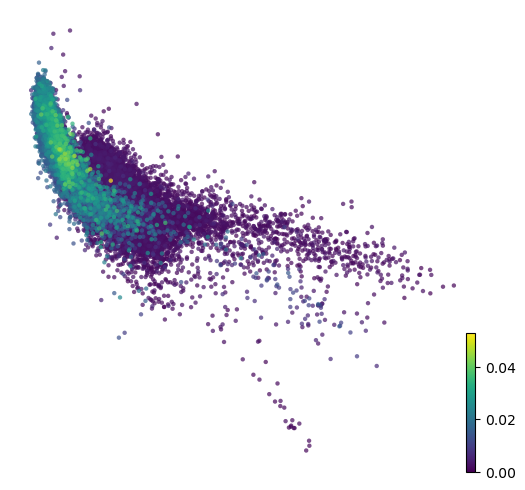
# Scatter plot of uncertainty vs. latent time colored by cell cycle phase
fig, ax = plt.subplots(figsize=(6, 6))
scv.pl.scatter(adata, y='diff_entropy', x='vae_time', color='CellCycle', size=40, alpha=0.7, ax=ax, legend_loc='right', frameon=False, title='');
Save the final result
[21]:
adata.write_h5ad(data_path_base+"/final.h5ad")
[ ]: